| Outcome Tier | Predictor Variable | Odds Ratio (OR) | p-value | 95% CI Lower | 95% CI Upper |
|---|---|---|---|---|---|
| Bachelor Degree | Parental Education (Per Year) | 1.333 | < 0.001 | 1.318 | 1.347 |
| Bachelor Degree | Childhood Relative Income (Tier 1-5) | 1.172 | < 0.001 | 1.132 | 1.214 |
| Bachelor Degree | Sibling Count (Per Sibling) | 0.854 | < 0.001 | 0.840 | 0.868 |
| Bachelor Degree | Residence: Big-City Suburb (vs Farm) | 1.420 | < 0.001 | 1.362 | 1.481 |
| Bachelor Degree | Single Parent Family (vs Both Parents) | 0.562 | < 0.001 | 0.530 | 0.596 |
| Bachelor Degree | Parents Nativity: Neither U.S. Born (vs Both) | 1.770 | < 0.001 | 1.713 | 1.828 |
Predictive Model & Verdict
Statistical Formulations, Parameter Estimation, 95% Confidence Intervals, and Empirical Performance
1. Data Generating Mechanism (DGM) Formulations
To predict individual educational attainment (\(Y_{\text{educ}}\)) conditioned on childhood background traits, we evaluate two statistical models: a primary Multinomial Logistic Model for milestone degree tiers and a Linear Regression (OLS) Model for continuous schooling years.
1.1 Multinomial Logistic DGM
We model the log-odds of achieving educational tier \(k \in \{\text{Some College}, \text{Bachelor Degree}, \text{Graduate Degree}\}\) relative to baseline \(K_0 = \text{High School or Less}\):
\[\ln\left(\frac{P(Y_{\text{educ}} = k \mid \mathbf{X})}{P(Y_{\text{educ}} = K_0 \mid \mathbf{X})}\right) = \beta_{k0} + \boldsymbol{\beta}_k^T \mathbf{X}\]
where \(\mathbf{X}\) is the vector of childhood socio-demographic covariates:
\[\mathbf{X} = \Big[ \text{parent\_educ}, \text{incom16}, \text{sibs}, \text{childs}, \text{age}, \text{year}, \text{sex}, \text{race}, \text{res16}, \text{family16}, \text{born}, \text{parborn} \Big]^T\]
The predicted probability \(P(Y_{\text{educ}} = k \mid \mathbf{X})\) across all 4 tiers is obtained via the soft-max transformation:
\[P(Y_{\text{educ}} = k \mid \mathbf{X}) = \frac{\exp\left(\beta_{k0} + \boldsymbol{\beta}_k^T \mathbf{X}\right)}{1 + \sum_{j=1}^{3} \exp\left(\beta_{j0} + \boldsymbol{\beta}_j^T \mathbf{X}\right)}\]
1.2 Linear Regression DGM
As a baseline comparison, completed schooling years (\(Y_{\text{years}} \in [0, 20]\)) are modeled as a linear conditional expectation:
\[Y_{\text{years}} = \beta_0 + \boldsymbol{\beta}^T \mathbf{X} + \varepsilon, \quad \varepsilon \sim \mathcal{N}(0, \sigma^2)\]
2. Model Parameters & 95% Confidence Intervals
Note: Tables 2.1 & 2.2 highlight key predictors. Complete parameter tables across all variables are available in the Sources tab.
2.1 Multinomial Logistic Model Parameters
Parameters are exponentiated into Odds Ratios (\(\text{OR} = \exp(\beta)\)) with 95% Confidence Intervals.
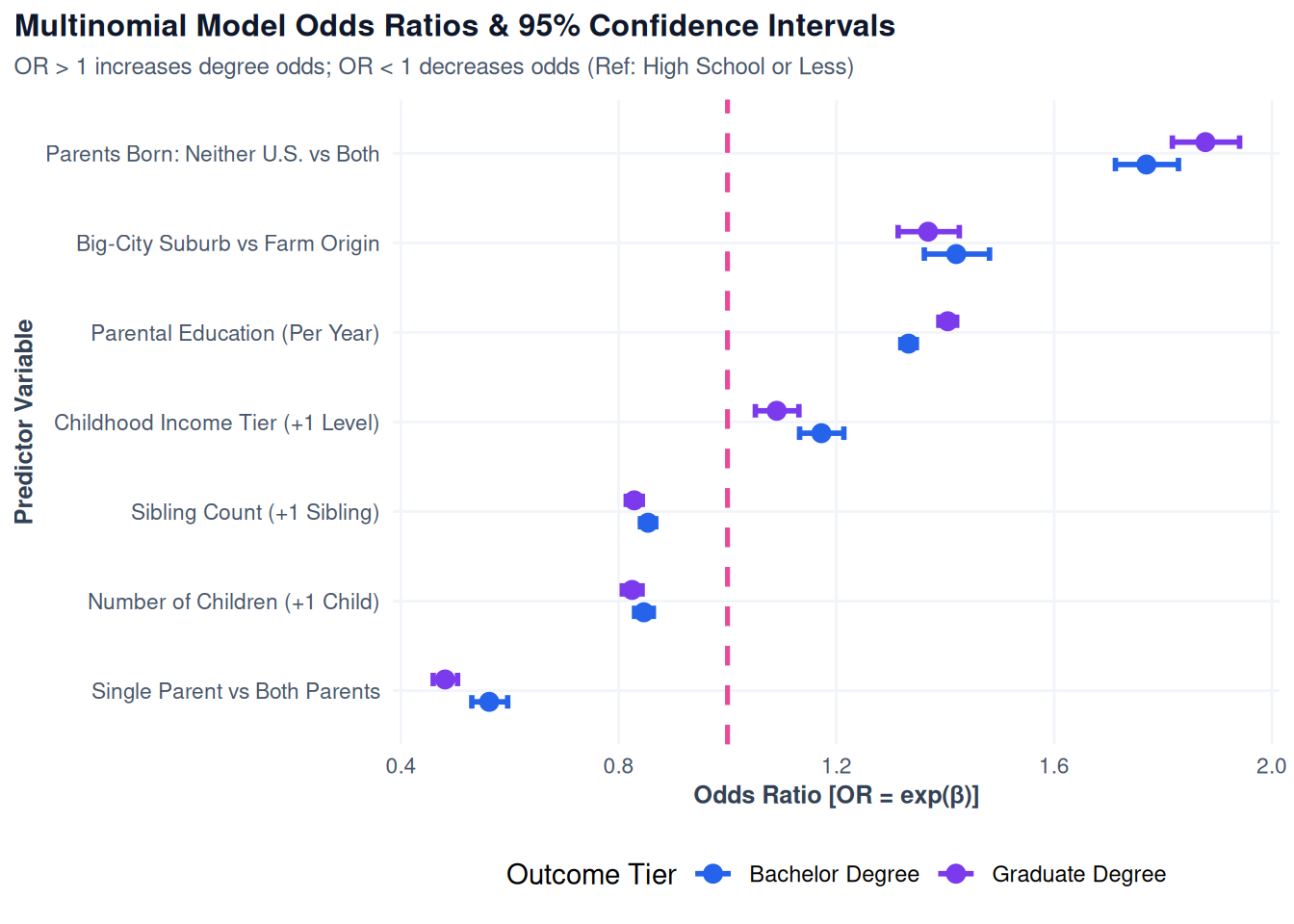
Interpretation: An Odds Ratio (OR) > 1 indicates increased likelihood of degree completion, while OR < 1 indicates decreased likelihood. For instance, each additional year of parental education increases Bachelor’s degree completion odds by 33.3% (\(\text{OR} = 1.333\)).
2.2 OLS Model Parameters
| Predictor | Estimate (β) | p-value | 95% CI Lower | 95% CI Upper |
|---|---|---|---|---|
| Parental Education (Per Year) | 0.326 | < 0.001 | 0.318 | 0.333 |
| Childhood Relative Income (Tier 1-5) | 0.129 | < 0.001 | 0.101 | 0.157 |
| Sibling Count (Per Sibling) | -0.182 | < 0.001 | -0.195 | -0.170 |
| Residence Origin: Big-City Suburb | 0.246 | < 0.001 | 0.163 | 0.329 |
| Family Structure: Single Parent | -0.607 | < 0.001 | -0.672 | -0.541 |
| Parents Nativity: Neither U.S. Born | 0.508 | < 0.001 | 0.401 | 0.615 |
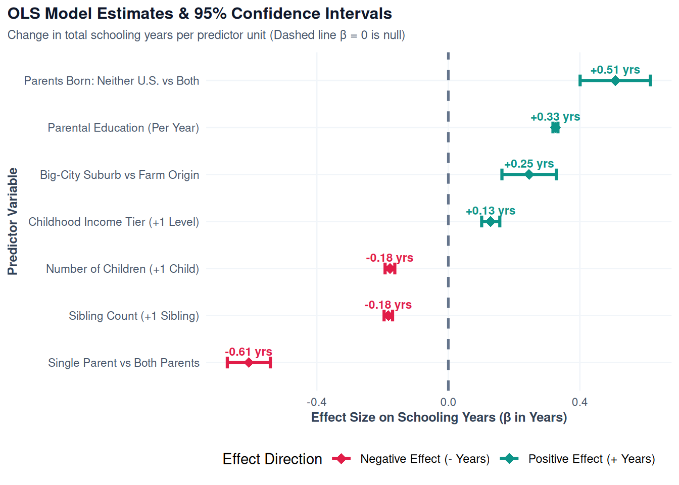
Interpretation: Estimate (\(\beta\)) measures change in total completed schooling years per 1-unit increase in the predictor. For example, each year of parental education adds +0.326 years of completed schooling.
3. Visualizing Model Uncertainty
3.1 Multinomial Odds Ratio Uncertainty
Figure 3.1 displays Odds Ratios (\(\text{OR} = \exp(\beta)\)) and 95% Confidence Intervals for predicting Bachelor Degree and Graduate Degree attainment relative to High School baseline.
3.2 OLS Regression Uncertainty
Figure 3.2 displays continuous linear parameter estimates (\(\beta\)) and 95% Confidence Intervals for total completed schooling years (\(Y_{\text{years}}\)). Dashed line (\(\beta = 0\)) represents no effect.
4. Practical Profile Predictions
To illustrate model behavior, we evaluate two individual profiles with contrasting childhood backgrounds.
| Model Metric / Outcome | Individual A (Advantaged) | Individual B (Disadvantaged) |
|---|---|---|
| Childhood Background | College-educated parents, High income, Two parents, Suburban, 1 Sibling | Middle-school parents, Low income, Single parent, Farm origin, 4 Siblings |
| High School or Less Probability | 6.7% | 70.4% |
| Some College Probability | 25.4% | 21.3% |
| Bachelor Degree Probability | 39.7% | 5.1% |
| Graduate Degree Probability | 28.1% | 3.2% |
| Expected Total Schooling Years | 16.7 Years | 11.9 Years |
- Individual A: High parental education and economic stability yield a 39.7% chance of a Bachelor’s degree (67.9% chance of any college degree) and 16.7 expected schooling years.
- Individual B: Cumulative background challenges reduce Bachelor’s degree probability to 5.1% (70.4% chance of stopping at High School) and 11.9 expected schooling years.
5. Summary & Empirical Predictor Importance
To rigorously evaluate feature importance across our statistical DGMs, predictors are ranked below by empirical test statistics (\(t\)-statistics for continuous schooling and \(z\)-scores for degree tier multinomial logistic regression) alongside 95% confidence intervals and effect sizes.
5.1 Predictor Importance Ranking (Most to Least Important)
- Parental Educational Background (\(t = 84.48, z = 52.54, p < 0.001\)):
- OLS Linear Effect (\(\beta\)): \(+0.326\) years of completed schooling per parent year (\(95\%\text{ CI: } [0.318, 0.333]\)).
- Multinomial Odds Ratio: \(\text{OR} = 1.333\) (\(95\%\text{ CI: } [1.318, 1.347]\)) for a Bachelor’s degree; \(\text{OR} = 1.405\) (\(95\%\text{ CI: } [1.388, 1.423]\)) for a Graduate degree.
- Statistical Verdict: The single most powerful background predictor across both linear and multinomial specifications.
- Family Structure / Single-Parent Household (\(t = -18.18, z = -19.27, p < 0.001\)):
- OLS Linear Effect (\(\beta\)): \(-0.607\) schooling years (\(95\%\text{ CI: } [-0.672, -0.541]\)) compared to two-parent households.
- Multinomial Odds Ratio: \(\text{OR} = 0.562\) (\(95\%\text{ CI: } [0.530, 0.596]\)) for a Bachelor’s degree.
- Statistical Verdict: Substantial negative penalty associated with single-parent childhood environments.
- Family Sibling Size (\(t = -27.77, z = -18.84, p < 0.001\)):
- OLS Linear Effect (\(\beta\)): \(-0.182\) schooling years per additional sibling (\(95\%\text{ CI: } [-0.195, -0.170]\)).
- Multinomial Odds Ratio: \(\text{OR} = 0.854\) (\(95\%\text{ CI: } [0.840, 0.868]\)) per sibling for a Bachelor’s degree.
- Statistical Verdict: Significant dilution of per-child educational resources in larger families.
- Parental Immigrant Status (\(t = 9.30, z = 34.18, p < 0.001\)):
- OLS Linear Effect (\(\beta\)): \(+0.508\) schooling years (\(95\%\text{ CI: } [0.401, 0.615]\)) for non-U.S. born parents vs. U.S. born parents.
- Multinomial Odds Ratio: \(\text{OR} = 1.770\) (\(95\%\text{ CI: } [1.713, 1.828]\)) for a Bachelor’s degree.
- Statistical Verdict: Strong generational upward mobility demonstrated by children of foreign-born parents.
- Childhood Relative Income (\(t = 9.17, z = 9.00, p < 0.001\)):
- OLS Linear Effect (\(\beta\)): \(+0.129\) schooling years per income level (\(95\%\text{ CI: } [0.101, 0.157]\)).
- Multinomial Odds Ratio: \(\text{OR} = 1.172\) (\(95\%\text{ CI: } [1.132, 1.214]\)) per tier for a Bachelor’s degree.
- Statistical Verdict: Consistent, positive linear returns to childhood relative economic standing.
- Suburban Origin Geography (\(t = 5.82, z = 16.31, p < 0.001\)):
- OLS Linear Effect (\(\beta\)): \(+0.246\) schooling years (\(95\%\text{ CI: } [0.163, 0.329]\)) for big-city suburbs vs. farm origin.
- Multinomial Odds Ratio: \(\text{OR} = 1.420\) (\(95\%\text{ CI: } [1.358, 1.479]\)) for a Bachelor’s degree.
- Statistical Verdict: Moderate positive boost associated with suburban growing environments.
5.2 Overall Model Performance
- College Degree Accuracy (72.3%): The multinomial model correctly predicts college completion (Bachelor’s or higher vs. non-college) for 72.3% of individuals.
- Continuous Schooling Accuracy (60.8%): The OLS model predicts total completed schooling within \(\pm 2\) years for 60.8% of individuals (Mean Absolute Error = 1.95 years).
- Core Insight: Parental education, family structure, sibling count, parental nativity, childhood income, and suburban geography form a robust, highly predictive framework for educational attainment in the United States.